Blended TPW Products AlgorithmThis page contains simple descriptions of the blending algorithms used for the blended TPW products. More details please refer to Kidder and Jones. 1. Over Ocean Algorithm1.1 Histogram Correction
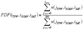
The first step in the ocean blending algorithm is the construction of histograms of TPW
values for a five-day period. A histogram is constructed for each satellite instrument
at each scan position. The assumption is that in a five-day period, each scan position
of each instrument will sample the global distribution of TPW.
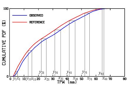
The second step in the process is constructing a reference PDF. While the "true" TPW distribution is not known, one set of observations can be chosen to be the reference and an adjustment can be calculated. When the adjustment is applied to other observations it makes the distribution approximate the reference distribution. Currently the average TPW PDF of the Suomi-NPP ATMS instrument is used as the reference PDF. Figure1 shows an example of the reference for the five day period as the red line.
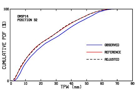
Figure 1. Illustration of the blending algorithm. [From K&J Fig. 1.]The third step in the process is the construction of an adjustment for each scan position of each instrument. The blue line in Fig. 1 shows the cumulative PDF for scan position 32 on the DMSP F14 SSM/I for the time period above. The TPW histograms are tabulated with 1-mm-width bins centered at 0.5 mm, 1.5 mm, etc. For each bin from 5.5 mm to 68.5 mm (the 64 xi values) a yi is interpolated such that the observed cumulative PDF has the same value as the cumulative reference PDF. This step is illustrated in Fig. 1 for a subset of the xi and yi values. Then, applying the adjustment is just a simple process of selecting the coefficients (as a function of satellite and scan position), using the observed TPW as x, and calculating y: adjusted TPW = a0 + a1TPW + a2TPW2 + a3TPW3 (2)Figure 2 shows the adjusted cumulative PDF (dashed line) for the data shown in Fig. 1.
Figure 2. The dashed line shows the results of adjusting the observed TPW
data with the blending algorithm.
|
|||||||||||||||||
| Table 1. Current Barnes analysis parameters for GPS data. | |
|---|---|
| Barnes Analysis Parameter | Value |
| Minimum number of GPS data points within range for Barnes analysis to proceed | 3 |
| 1/e decay length | 250 km |
| Maximum number of stations in an analysis | 100 stations |
| Maximum distance of closest station | 300 km |
| Maximum distance of a station to consider (stations further than this not used) | 600 km |
| Condition to extend a single station analysis |
< 8 points within 600 km and nearest within 50 km of point-in-question. |
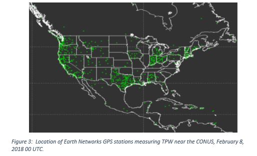
A land mask is used to only add GPS data over land. No averaging or error-weighting of the microwave and GPS data is currently performed, although such approaches are worthy of further study.
The GOES Sounder data are mapped directly into the Mercator projection, and then a 3 x 3 grid box expansion is performed, or up to roughly a 48 km2 areal coverage. This is strictly to eliminate holes in the analysis from insufficient coverage of the gridded data. In the future, the GOES Sounder results could be remapped or averaged together to eliminate missing values.
In order to augment the global TPW product with GPS and GOES data, at each point, the TPW value is selected in the following order:
The search for a TPW value ends as soon as one is found, so that the blended TPW values over ocean remind unchanged, and GPS data are selected preferentially over GOES PW values. No averaging or error-weighting of the data is currently performed, although such approaches are worthy of further study.
To give forecasters an idea about how abnormally moist or dry the Blended TPW Product is, the TPW values from the blended product are divided by the weekly mean TPW values from the NVAP Dataset for 1988-1999 (Randel et al. 1996). NVAP is a daily, 1-degree resolution analysis which was created with TPW derived from SSM/I (ocean), NOAA TOVS (ocean and land), and radiosonde (land). This gives "percent of normal." There are 52 weekly mean fields used as normal from NVAP. No moving mean or 3-1-3 (three days before, the current day, and the next three days) calculation of the weekly mean is currently performed. The percent of normal product was developed at CIRA for research purposes but has proven useful for tracking atmospheric rivers, return flow of moisture from the Gulf of Mexico, and abnormally dry conditions associated with fire danger.
A new Cylindrical map is also added in June of 2019 when the product are updated to include NOAA-20 TPW retrievals while the blended TPW and Percentage of TPW Normal products are written out as netCDF formats.
For more details about the blending algorithm, see cat.cira.colostate.edu/kidder/Blended_TPW.pdf.