Blended TPW Products Algorithm
This page contains simple descriptions of the blending algorithms used for the blended
TPW products. More details please refer to Kidder
and Jones.
1. Over Ocean Algorithm
1.1 Histogram Correction
The first step in the ocean blending algorithm is the construction of histograms of TPW
values for a five-day period. A histogram is constructed for each satellite instrument
at each scan position. The assumption is that in a five-day period, each scan position
of each instrument will sample the global distribution of TPW.
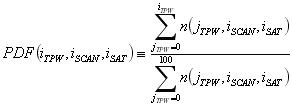
Let n(iTPW, iSCAN, iSAT) be the five-day histogram,
where iTPW is the integral value of the retrieved
TPW value in millimeters (range: 0-100),
iSCAN is the scan position, and iSAT is the index for the
satellite (range: 1 to nsat).
The cumulative probability distribution function is defined as, where PDF ranges from
zero to one.
The second step in the process is constructing a reference PDF. While the "true" TPW
distribution is not known, one set of observations can be chosen to be the reference and
an adjustment can be calculated. When the adjustment is applied to other observations it
makes the distribution approximate the reference distribution. Currently the average TPW
PDF of the Suomi-NPP ATMS instrument is used as the reference PDF. Figure1 shows an
example of the reference for the five day period as the red line.
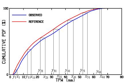
Figure 1. Illustration of the blending algorithm. [From K&J Fig. 1.]
The third step in the process is the construction of an adjustment for each scan
position of each instrument. The blue line in Fig. 1 shows the cumulative PDF for scan
position 32 on the DMSP F14 SSM/I for the time period above. The TPW histograms are
tabulated with 1-mm-width bins centered at 0.5 mm, 1.5 mm, etc. For each bin from 5.5 mm
to 68.5 mm (the 64 xi values) a yi is interpolated such that the observed cumulative PDF
has the same value as the cumulative reference PDF. This step is illustrated in Fig. 1
for a subset of the xi and yi values. Then, applying the adjustment is just a simple
process of selecting the coefficients (as a function of satellite and scan position),
using the observed TPW as x, and calculating y:
adjusted TPW = a0 + a1TPW +
a2TPW2 + a3TPW3 (2)
Figure 2 shows the adjusted cumulative PDF (dashed line) for the data shown in Fig. 1.
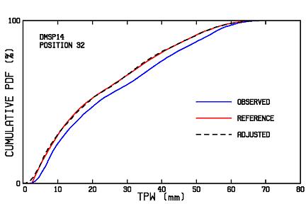
Figure 2. The dashed line shows the results of adjusting the observed TPW
data with the blending algorithm.
[From K&J Fig. 2.]
It is worth to mention that the Ocean blending algorithm has been applied over both
Ocean and Land since the TPW retrievals were available from MiRS in since 2011.
1.2 Remapping
Each orbit of satellites is corrected with the histogram matching method and then mapped
with a chosen map projection. The base map was chosen to be compatible with a map used
at NESDIS/SAB. It is a Mercator projection with 16 km resolution at the equator. The map
is centered at the equator and 160° west. It has 1437 rows and 2500 columns. The upper
left pixel is at 71°14'52" North, 20°20'38" East, and the lower right pixel is at
71°14'52" South, 19°35'3" East. The cut line is at 20° East, which was chosen to
emphasize ocean areas. Each orbit of each satellite is corrected with the histogram
matching method and mapped onto the output map.
1.3 Compositing
Satellite data may be composited or blended in a variety of ways depending on the
intended use of the blended product. The most common way to blend data is to average
them over a specified time period, and another way is to overlay newer data on top of
older data, such that only the newest data are displayed. The overlay method of
compositing is favored by forecasters because it is the most up-to-date image possible,
and is used for the current operational TPW products. The orbits for the 12-hour period
prior to runtime are composited by overlaying newer pixels on top of older pixels.
2. Over Land Algorithm
Two additional data sources are currently used in the over-Land algorithm: (1)
ground-based GPS TPW retrievals; (2) PW (layered and total) retrievals from the GOES.
Those data are available only over the CONUS, with a few stations in Alaska, Hawaii,
Puerto Rico, Mexico and Canada; The basic plan for the current over-Land algorithm is to
overlay the MIRS retrievals with the GPS retrievals when they are available, then use
the GOES TPW to fill the left “holes” when no GPS and MIRS retrievals are available. GPS
data are used in preference to the GOES PW data because GPS TPW values are unaffected by
clouds, whereas GOES PW values can be retrieved only in cloud-free conditions.
Passive microwave retrievals over Land are used first and serve as the primary TPW value
if no other data will be available and overlay them. Over OCUNUS, GPS TPW retrievals are
overlaid as a first priority, if they pass tests for sufficient data density and
allowable distance from the point in question. Then GOES TPW are used when there are
still missing data voids. The GOES PW data provide a valuable backup in case the GPS
data are not available. Historically, GOES Sounders from GOES-13/-15 were used in the
blended TPW, but as of June of 2019, only GOES-15 data is available, which will be gone
soon when the GOES-15 is terminated. Research is in progress to incorporate the GOES-R
series of satellites TPW retrievals.
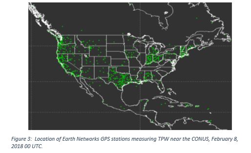
Typical coverage of the GPS network is shown in Figure 3. The Barnes analysis
interpolation parameters for GPS are shown in Table 1 and further described below. In
practice, GPS makes large contributions over most of the CONUS, but has minimal impact
over Canada and Mexico due to sparse station coverage. In the GPS-sparse northern
plains, GPS data is usually not sufficient and the microwave retrievals are compose the
solution.
A Barnes analysis (Barnes 1964, Koch et al. 1983) of the GPS data is performed to create
a smooth field. The Barnes analysis approach has several parameters which must be
specified, relating to the spatial influence of the data. Table 1 lists the values used
in the Barnes analysis of the GPS TPW data. The values chosen are rather liberal (e.g.
allowing an analysis up to 300 km from the nearest station) and geared towards a smooth
field and high spatial coverage over CONUS. These values could be modified in the future
to emphasize for instance increased spatial structure at the expense of high coverage.
In regions with only a few stations in the Barnes analysis (e.g. Mexico, southern
Canada), a circular feature can be produced in the analysis as only a few stations are
available for interpolation and data points exceed the distance criteria in Table 1.
| Table 1. Current Barnes analysis parameters for GPS data. |
| Barnes Analysis Parameter |
Value |
| Minimum number of GPS data points within range for Barnes analysis to proceed
|
3 |
| 1/e decay length |
250 km |
| Maximum number of stations in an analysis |
100 stations |
| Maximum distance of closest station |
300 km |
| Maximum distance of a station to consider (stations further than this not used)
|
600 km |
| Condition to extend a single station analysis |
< 8 points within 600 km and nearest
within 50 km of point-in-question.
|
A land mask is used to only add GPS data over land. No averaging or error-weighting of
the microwave and GPS data is currently performed, although such approaches are worthy
of further study.
The GOES Sounder data are mapped directly into the Mercator projection, and then a 3 x 3
grid box expansion is performed,
or up to roughly a 48 km2 areal coverage. This is strictly to eliminate holes
in the analysis from insufficient coverage of the gridded data.
In the future, the GOES Sounder results could be remapped or averaged together to
eliminate missing values.
In order to augment the global TPW product with GPS and GOES data, at each point, the
TPW value is selected in the following order:
1. The TPW values from satellite microwave retrievals (if present, no other data are
available)
2. The GPS TPW values from the Barnes analysis (if present, using the GPS data to
overlay the microwave retrievals)
3. The GOES TPW value (if present)
The search for a TPW value ends as soon as one is found, so that the blended TPW values
over ocean remind unchanged, and GPS data are selected preferentially over GOES PW
values. No averaging or error-weighting of the data is currently performed, although
such approaches are worthy of further study.
3. TPW Anomaly (Percentage of Normal)
To give forecasters an idea about how abnormally moist or dry the Blended TPW Product
is, the TPW values from the blended product are divided by the weekly mean TPW values
from the NVAP Dataset for 1988-1999 (Randel et al. 1996). NVAP is a daily, 1-degree
resolution analysis which was created with TPW derived from SSM/I (ocean), NOAA TOVS
(ocean and land), and radiosonde (land). This gives "percent of normal." There are 52
weekly mean fields used as normal from NVAP. No moving mean or 3-1-3 (three days before,
the current day, and the next three days) calculation of the weekly mean is currently
performed. The percent of normal product was developed at CIRA for research purposes but
has proven useful for tracking atmospheric rivers, return flow of moisture from the Gulf
of America, and abnormally dry conditions associated with fire danger.
4. netCDF format
A new Cylindrical map is also added in June of 2019 when the product are updated to
include NOAA-20 TPW retrievals while the blended TPW and Percentage of TPW Normal
products are written out as netCDF formats.
For more details about the blending algorithm, see
cat.cira.colostate.edu/kidder/Blended_TPW.pdf.
